
Introduction
The studio now has an honest prediction boundary. Does a small regression model improve its material-planning estimate over an earlier attendance median? You will fit a short Pipeline, compare both methods on the same labeled workshops and save a real comparison image plus future predictions.
You need Python functions, pandas selection and joins, basic Scikit-learn regression/train-test concepts and introductory Matplotlib. The previous Guided Lab explains the seven-day deadline and training-only imputation. This lab independently prepares all files, including the completed ID/date split; no previous VM files are needed. All data is original synthetic teaching material. The 60-minute duration is an author estimate.
Fit a Small Pipeline on Earlier Workshops
In this step, you will move from a training-median baseline to a reusable feature-based seven-day predictor.
Open the WebIDE Tab. In File > Open Folder, open /home/labex/project/workshop-attendance. The Explorer file tree shows the source modules and CSV inputs together. Select a filename to read it; use Edit > Find to find a function name such as fit_model. Python indentation groups statements: keep the four spaces inside a function. After an edit, choose File > Save before running it. An unsaved editor buffer does not change what Python reads.
Use the separate Terminal Tab for the commands below; return to WebIDE when asked to edit. The course's ./python launcher selects its prepared scientific environment. Do not use the editor's default Run button or change its interpreter to repair a course command. cd changes only this terminal's working directory; a reopened terminal needs its own cd. Opening either entry never installs or resets the scene.
The Results Tab reads only actual saved files under output/. All files / Refresh reads current files, View opens one artifact, and Download returns its original bytes. Missing files remain missing: Results never runs analysis, fills results or redraws charts. Return to Terminal before commands.
cd /home/labex/project/workshop-attendance
cat displays files without editing them; multiple filename arguments display them one after another.
cat season.json history.csv labels.csv future.csv
Each historical row is a workshop keyed by session_id. labels.csv associates actual_attendance by that key, in an independent order. The only allowed numeric model features are booked_7d, a snapshot saved exactly seven days before the event, and duration_minutes, already announced at that deadline. Blank numeric cells mean missing information; each allowed feature has a nonempty training observation. IDs and dates are for association and separation, not model inputs. final_bookings and scanned_entries happen at the event and leak information unavailable seven days earlier.
The completed split freezes training at April 1, 2026 at 00:00 UTC and reserves historical events from April 12 onward for evaluation. Training labels are known by the end of each earlier event day; the final training event here is March 8. The earliest holdout prediction happens April 5, using that event's own seven-day snapshot with the model already frozen. April 5 input is not claimed to be available on April 1. Later snapshot files replay the corresponding later prediction dates. future.csv has no actual labels; its May events get predictions, not measured errors. There are no historical rows in the configured gap. The course does not cover rolling refits or all-empty training features.
cat split.py
Observe its key-based merge, parsed calendar boundaries and date sorting. It is the completed split from the previous lesson, supplied here for independence. Preserve it, all CSV/JSON inputs, python, run.py, coursekit.py, show_results.py and the starter-*.py files. Edit model.py, chart.py and your output/ artifacts only. The supplied model.py starts with a deliberately limited training-median predictor. It uses no post-event inputs. A tempting alternative would fit train[["scanned_entries"]]: those scans exist only after the event, so perfect historical-looking numbers would not rescue that invalid information choice.
A Pipeline chains preprocessing and a model. During fit, its imputer learns means from the provided training features, then its regression learns from the filled training matrix. During predict, the same imputer only transforms the later inputs. It never fits again on the holdout or future. LinearRegression fits an intercept and feature coefficients by ordinary least squares; we keep this small model instead of tuning many alternatives.
First run the limited starter, before editing. In model.py, DummyRegressor(strategy="median") learns only a training-target median; its dummy zero column is not a workshop feature. It predicts the same count for every row. This establishes a real baseline, not a fitted feature-based regression.
./python run.py fit
./python show_results.py fit
Both model_prediction and baseline_prediction in this preview are 24.5 for each supplied holdout ID. The runner keeps its stable column names; here the candidate in the model column is baseline-only. The fit check must still reject this incomplete workflow on informative inputs. A valid fitted regression with zero coefficients can also be constant on other data; constancy alone is not a universal error.
Open run.py to follow the call from split_events to fit_model and then predict_events; return to model.py to edit. FEATURES is exactly ['booked_7d', 'duration_minutes']. The imports are already supplied. The existing correct evaluate below these functions will be read in the next step; leave it unchanged.
Return to Terminal before making the backup.
cp model.py model.py.bak
In WebIDE replace only the bodies of fit_model and predict_events with those shown below; keep their signatures, imports and the supplied evaluate. fit_model returns the fitted estimator and the training-target median. predict_events selects the same permitted columns for each input table.
def fit_model(train):
    model = make_pipeline(SimpleImputer(strategy="mean"), LinearRegression())
    model.fit(train[FEATURES], train.actual_attendance)
    return model, float(train.actual_attendance.median())


def predict_events(model, events):
    return model.predict(events[FEATURES])
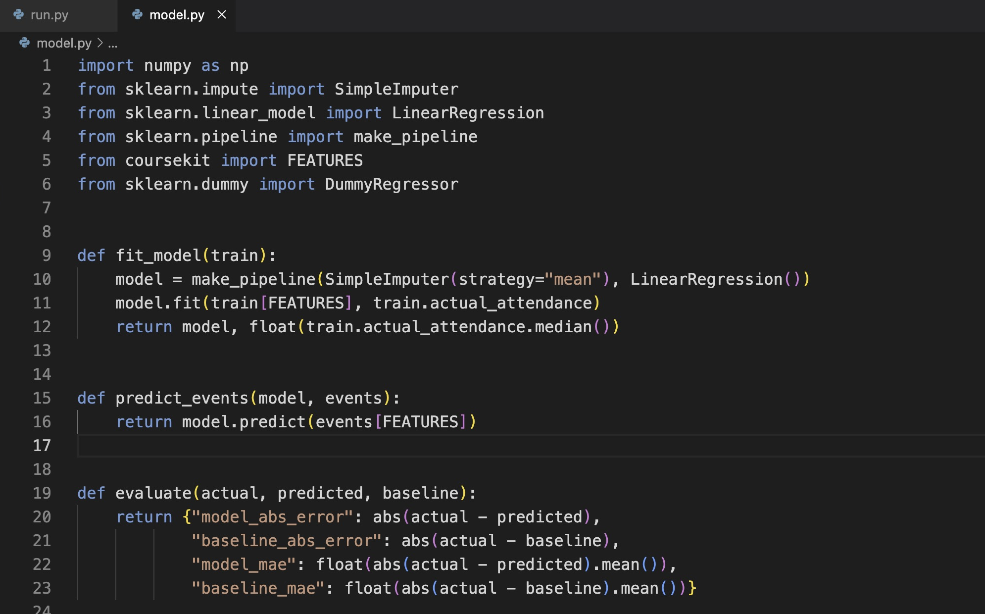
The edited model uses only FEATURES for fitting and prediction. Keep the supplied evaluate function below unchanged, save model.py, then return to Terminal.
Save the file, return to Terminal and rerun the preview.
./python run.py fit
./python show_results.py fit
The saved preview should associate W-88 with a raw prediction near 32.718, actual attendance 46 and baseline 24.5; W-09 should have prediction near 62.236, actual 74 and the same baseline. A regression output can be fractional even though one actual workshop admits a whole number of people.
These are predictions before error summarization. They were fitted without the later labels. Changing those labels should change the eventual errors, not the fitted predictions. A feature with zero learned coefficient may legitimately have no influence; changing any arbitrary input does not necessarily change a prediction.
Compare Continuous Errors on the Same Holdout
In this step, you will compute absolute errors from real holdout labels and compare their means in people.
Continue in the Terminal Tab at /home/labex/project/workshop-attendance. An absolute error is the magnitude of actual - predicted. np.abs computes it element by element; np.mean averages the resulting array. For a fair baseline, subtract the same earlier target median from each of the same actual holdout labels. Never compare different event sets or substitute a prediction for an actual outcome.
Use the raw continuous predictions for all errors and MAEs. Rounding a prediction to a displayed head count first changes the evaluation. The wrapper will format console MAE to three decimal places for reading while saving the unrounded numeric value in JSON.
Open model.py in WebIDE and find the supplied evaluate(actual, predicted, baseline). This function was already correct at initialization; keep it unchanged. It returns absolute-error arrays and their means. There is no empty error function to fill and no reason to overwrite your completed model functions.
Follow the four returned keys. For W-88, use its actual 46, raw model estimate near 32.7176 and training median 24.5 to predict which of the two absolute errors is smaller. The existing abs works element by element on the runner's NumPy arrays; taking each array's .mean() then converting to float gives a JSON-compatible number. np.abs and np.mean are equivalent NumPy forms, not required edits.
The wrapper preserves the same holdout rows' IDs when saving output/holdout.csv. Error vectors follow the supplied arrays' position order. Equivalent array-like returns, including pandas Series, are accepted in that order; numeric Series index labels are not workshop IDs. Return to Terminal to calculate and read the real comparison. After the corrected step-1 model, this step's check may already pass because the error function was supplied; read and verify what it computes rather than deleting it to manufacture work.
./python run.py evaluate
Expected console summary:
Model MAE (people): 12.523
Baseline MAE (people): 35.500
./python show_results.py evaluate
For W-88, the model error is about 13.282 people and the baseline error is 21.5. For W-09, they are about 11.764 and 49.5. The unrounded means are approximately 12.5230751656 and exactly 35.5 people. The earlier warmup baseline was 18; this full season's training median is 24.5 because it uses a different early sample.
Here the small model has a lower error on these two held-out events. That is evidence about this small synthetic holdout, not proof of future reliability or an effect caused by bookings. If a correct model instead has higher MAE, the honest conclusion is that it did not improve this comparison. Assessment never requires the model to beat the baseline, and constant or uninformative features are legitimate.
Deliver the Chart and Unlabeled Forecasts
In this step, you will make the holdout comparison readable and export future estimates without inventing actual outcomes.
Continue in the Terminal Tab at /home/labex/project/workshop-attendance. Your chart must plot one value per held-out ID for each of the series Actual, Model and Baseline, using the raw people values from the comparison table. A line or scatter plot is suitable; labels and IDs keep its meaning clear. The PNG must be readable, at least 600 by 300 pixels, and reproduce the same visible chart when rerun on the same data. Styling may differ. Assessment checks actual plotted values and the saved image, not a self-reported chart manifest. Every business point must remain within the visible axes limits, and no required series may be hidden or fully transparent. Points exactly on a limit are allowed; colors and axis ranges may differ.
Matplotlib's Agg backend writes an image without opening a desktop window. subplots creates a figure and axes; plot draws each ID-linked series. The marker strings below distinguish hollow actual circles, model diamonds and dashed baseline crosses, including when actual and baseline overlap. tight_layout reserves room for labels. savefig writes the real PNG and close releases the figure.
Return to WebIDE and open chart.py. Imports, a figure, axes labels and the save/close lifecycle are already prepared. Find the marked series region: it currently raises NotImplementedError, so an attempted delivery cannot produce a completed comparison image. Keep the surrounding frame.
Return to Terminal for the backup command.
cp chart.py chart.py.bak
Return to WebIDE. Replace only the marked region's raise NotImplementedError(...) statement with this data binding. Each row supplies its own stable ID and three actual saved numeric values; do not hardcode the example counts.
    ids = result.session_id
    ax.plot(ids, result.actual_attendance, "o-", color="#2454a6",
            markerfacecolor="white", markersize=8, label="Actual")
    ax.plot(ids, result.model_prediction, "D-", color="#c66a19", label="Model")
    ax.plot(ids, result.baseline_prediction, "+--", color="#24815d",
            markersize=11, label="Baseline")
Save chart.py, then return to the Terminal Tab before running it. The destination passed to this function is where the existing frame saves your real chart. If a traceback points inside this block, check the field spelling and four-space indentation, save and rerun. cp chart.py.bak chart.py restores the original unfinished chart frame if needed without touching your completed model.
First practice a harmless spelling error. The next command intentionally uses an invalid stage name and exits with an argument error; it does not change your saved results.
./python run.py delvier
The message lists the allowed choices. Correct the spelling and run the delivery stage. If you get a file-not-found error instead, use pwd and ls, return with the initial cd command and try the correctly spelled filename.
./python run.py deliver
./python show_results.py deliver
The reader loads saved CSV/JSON and decodes the actual PNG; it never fills gaps from input data. Switch to Results, select All files / Refresh, then View beside output/comparison.png. The model should be below both actual attendance points; the baseline stays at 24.5. Different marker styles make equal-valued series distinguishable. Next select All files / Refresh, then View beside output/holdout.csv to compare the IDs and actual errors you just read on the chart. Return to the file list and view the PNG again if needed. Return to Terminal before the next command.

The supplied-data example shows actual attendance 46 and 74 at W-88 and W-09, model predictions near 32.718 and 62.236, and the dashed baseline at 24.5. The vertical separation from an actual point to its prediction represents that event's absolute error. Your styling may differ; the IDs and underlying values must agree.
forecast.csv contains only session_id, raw model_prediction and display_people. F-6 has a prediction near 19.119 and display count 19; F-101 has prediction near 25.245 and display count 25. For display only, the wrapper clips negative estimates to zero and rounds half upward using floor(max(raw, 0) + 0.5). This is a practical presentation rule, not a change to the evaluated model. The raw prediction is preserved even if it is negative or fractional.
No future actual count or future MAE is manufactured. A model may be frozen before a later prediction snapshot arrives: at each May event's seven-day deadline, reuse the existing model and that event's saved known features. Small synthetic samples, missing snapshots and changing attendance behavior limit what this analysis can support. The independent Challenge will change the season and dates while retaining this same workflow. Equivalent numerical implementations, output row orders and line/scatter styles are accepted with 1e-8 numeric tolerance and correct ID relationships.
If you restore model.py.bak, it returns to the limited median predictor, not the completed Pipeline. Re-edit only fit_model and predict_events, keep evaluate, save and rerun fit, evaluate and deliver. After any model edit, regenerate delivery before viewing the chart so the PNG and CSVs come from the same program.
Summary
You trained a small imputation/regression Pipeline on earlier workshops, compared its raw holdout errors with a training-median baseline and saved an ID-linked comparison chart. You also exported future estimates while keeping their unknown outcomes out of evaluation. A lower holdout MAE can support this limited comparison; a worse result is equally valid when it is computed honestly.